Q-SiMod
A typed metamodel for the model-driven engineering (MDE) of quantum simulation.
Quantum simulation lets a controllable quantum system stand in for a physical quantum system whose dynamics are classically intractable. In practice it is a chain of modelling steps: the Hamiltonian of a physical theory is subjected to truncations, changes of basis, encodings and perturbative mappings until it arrives at a hardware model, which is either analogue, meaning that a device realises the Hamiltonian natively, or digital, meaning a product formula to be executed on a gate-based quantum computer. Q-SiMod frames each of these steps as a transformation between typed artifacts. Every artifact carries a symbolic operator, a structural type and a parameter set; every transformation declares the structural types it requires and produces, whether it is exact or approximate, and its parameter relation. A pipeline of transformations is type-checked before anything is computed, the knob settings of a hardware model are found by a solver over the whole pipeline, and a numerical realisation layer validates the declarations by exact diagonalisation at small chain length.
The package implements the metamodel of the article it accompanies; see the citation.
Digital and analogue simulation
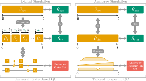
Both modes start from the same object: the dynamics of a physical system, governed by a
Hamiltonian \(\hat H_\text{sys}\) and carried out by the unitary \(\hat U_\text{sys}\) from the initial state at time \(0\)
to the target state at time \(t\). Digital simulation discretises that evolution into n
time slices, a Trotterisation, whose one- and two-qubit gates run on universal gate-based
hardware and realise an implicit, approximate Hamiltonian \(\hat H_\approx\). Analogue simulation maps
\(\hat H_\text{sys}\) onto a Hamiltonian \(\hat H_\text{sim}\) that a device realises natively and compiles it into
time-dependent control fields. Both chains terminate in an instruction set: a universal gate
set, portable across gate-based machines, or an analogue instruction set tailored to one
platform. The case study carries one physical theory down both branches, in the guide to the
lattice Schwinger model; the instruction sets themselves are out of scope.
The metamodel
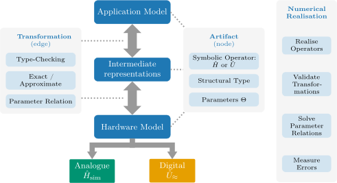
The chain of modelling steps is organised in three abstraction layers: an application model, the intermediate representations it passes through, and a hardware model, which simulates either in analogue mode, \(\hat H_\text{sim}\), or in digital mode, \(\hat U_\approx\). The nodes of that chain are the artifacts and its edges the transformations, with the attributes each of them declares shown beside them. Because artifacts and transformations are declarative, nothing is computed to type-check a pipeline; the numerical realisation layer on the right is separate and optional, and it is what realises the operators, validates the transformations, solves the parameter relations and measures the errors. The layers page names the module behind each of these boxes.
The model graph
Currently, three physical theories are implemented that descend from the application layer through intermediate representations to the hardware layer, and two of them arrive at the same hardware model. The figure shows the abstraction layers, the implemented artifacts and the transformations between them:
flowchart TB
subgraph LV1["Application model · <code>models.application</code>"]
direction LR
lattice_qed["<b>lattice_qed H<sub>sys</sub></b><br/>lattice QED<br/>(Kogut–Susskind)<br/><i>Θ<sub>sys</sub> = {m, a, e}</i>"]
xxz_magnet["<b>xxz_magnet H<sub>XXZ</sub></b><br/>Heisenberg XXZ magnet,<br/>by its anisotropy<br/><i>Θ = {J<sub>xy</sub>, Δ}</i>"]
ising_magnet["<b>ising_magnet H<sub>Ising</sub></b><br/>antiferromagnetic<br/>Ising chain<br/><i>Θ = {J<sub>z</sub>, h<sub>z</sub>, h<sub>x</sub>}</i>"]
end
subgraph LV2["Intermediate representations · <code>models.intermediate</code>"]
quantum_link_staggered["<b>quantum_link_staggered H<sub>IR1</sub></b><br/>quantum-link model,<br/>staggered mass<br/><i>Θ<sub>IR1</sub> = {m, κ}</i>"]
quantum_link_homogeneous["<b>quantum_link_homogeneous H<sub>IR2</sub></b><br/>quantum-link model,<br/>pair coupling<br/><i>Θ<sub>IR2</sub> = {m, κ}</i>"]
effective_bosonic["<b>effective_bosonic H<sub>IR3</sub></b><br/>boson encoding<br/><i>Θ<sub>IR3</sub> = {m, κ}</i>"]
qubit_register["<b>qubit_register H<sub>IR4</sub></b><br/>qubit Hamiltonian<br/><i>Θ<sub>IR4</sub> = {m, κ}</i>"]
xxz_chain["<b>xxz_chain H<sub>XXZ</sub></b><br/>XXZ chain,<br/>by its two couplings<br/><i>Θ = {J<sub>xy</sub>, J<sub>z</sub>}</i>"]
fermion_chain["<b>fermion_chain H<sub>tV</sub></b><br/>spinless fermions,<br/>nearest-neighbour interaction<br/><i>Θ = {J<sub>xy</sub>, J<sub>z</sub>}</i>"]
ising_chain["<b>ising_chain H<sub>Ising</sub></b><br/>Ising chain,<br/>by three energies<br/><i>Θ = {J<sub>z</sub>, Γ, B}</i>"]
end
subgraph LV3["Hardware model · <code>models.hardware</code>"]
direction LR
bose_hubbard["<b>bose_hubbard H<sub>sim</sub></b><br/>tilted, staggered<br/>Bose–Hubbard chain<br/><i>Θ<sub>sim</sub> = {J, U, δ, Δ}</i>"]
trotter["<b>trotter U<sub>≈</sub></b><br/>Trotter product formula<br/><i>t, n, order</i>"]
two_component_bose_hubbard["<b>two_component_bose_hubbard H<sub>2BHM</sub></b><br/>two-component<br/>Bose–Hubbard chain<br/><i>Θ = {t, U<sub>↑↑</sub>, U<sub>↑↓</sub>, U<sub>↓↓</sub>}</i>"]
end
subgraph OUT["Numerical realisation and solving"]
direction LR
SOLVE["<b>parameter realisation</b><br/>a constrained solve for the knob settings<br/>exact · approximate · infeasible · unsolved"]
VALID["<b>validity report</b><br/>every regime condition,<br/>with its margin"]
NUM["<b>numerical realisation</b><br/>dense operators in JAX,<br/>spectra and dynamics"]
SOLVE ~~~ VALID ~~~ NUM
end
L4(["Executable layer: gates, routing, pulses<br/><i>out of scope</i>"])
lattice_qed -. "<b>quantum-link truncation</b><br/><i>approximate, regime conditions</i>" .-> quantum_link_staggered
quantum_link_staggered ---> |"<b>particle–hole transformation</b><br/><i>exact</i>"| quantum_link_homogeneous
quantum_link_homogeneous ---> |"<b>boson encoding</b><br/><i>exact on the encoded subspace</i>"| effective_bosonic
effective_bosonic -. "<b>degenerate perturbation theory,<br/>solved for the knob settings</b><br/><i>approximate, regime conditions</i>" .-> bose_hubbard
quantum_link_homogeneous ---> |"<b>Jordan–Wigner transformation</b><br/><i>exact</i>"| qubit_register
qubit_register -. "<b>Trotterisation</b><br/><i>approximate, resource-controlled</i>" .-> trotter
xxz_magnet ---> |"<b>anisotropy resolution</b><br/><i>exact</i>"| xxz_chain
xxz_chain ---> |"<b>Jordan–Wigner to spinless fermions</b><br/><i>exact</i>"| fermion_chain
xxz_chain -. "<b>second-order superexchange,<br/>solved for the knob settings</b><br/><i>approximate, regime conditions</i>" .-> two_component_bose_hubbard
ising_magnet ---> |"<b>field resolution</b><br/><i>exact</i>"| ising_chain
ising_chain -. "<b>resonant dipole reduction,<br/>solved for the knob settings</b><br/><i>approximate, regime conditions</i>" .-> bose_hubbard
LV3 ==> |"a hardware model with bound parameters"| OUT
LV3 -.-> L4
classDef ham fill:#e0f2ee,stroke:#009371,color:#003e2f
classDef pf fill:#fbf1d9,stroke:#c48700,color:#573c00
classDef svc fill:#ede8f3,stroke:#988baa,color:#4c4655
classDef oos fill:#fdebea,stroke:#ed665a,color:#642b26
class lattice_qed,xxz_magnet,ising_magnet,quantum_link_staggered,quantum_link_homogeneous,effective_bosonic,qubit_register,xxz_chain,fermion_chain,ising_chain,bose_hubbard,two_component_bose_hubbard ham
class trotter pf
class SOLVE,VALID,NUM svc
class L4 oos
style LV1 fill:#f2f7fa,stroke:#b1d0e5,color:#103c5a
style LV2 fill:#f2f7fa,stroke:#b1d0e5,color:#103c5a
style LV3 fill:#f2f7fa,stroke:#b1d0e5,color:#103c5a
style OUT fill:#f6f4f9,stroke:#d8cee5,color:#5f576aA solid arrow is an exact transformation and a dotted arrow an approximate one, with
the kind of approximation in italics. Every artifact is built by the model library
(qsimod.models) and every transformation by the transformation library
(qsimod.transformations); the use cases assemble them into model
graphs:
qsimod.usecases.schwinger, the case study of the article: a one-dimensional lattice quantum electrodynamics (QED), carried to an analogue and a digital simulator model from a shared prefix.qsimod.usecases.heisenberg, an anisotropic Heisenberg magnet on a two-component optical lattice.qsimod.usecases.ising, an antiferromagnetic Ising chain on the hardware model of the case study.
Starting points
- One guide per application model, each walking through its pipeline artifact by artifact and transformation by transformation: the Hamiltonians, the structural types a transformation requires and declares, its validity conditions and the constants it discards. The guide to the lattice Schwinger model also introduces the machinery of the framework; the guides to the Heisenberg magnet and the Ising chain state what differs.
- The Layers of the package: which module constructs an operator and which imports a solver.
- The API reference, generated from the docstrings.
Citation
The package implements the metamodel of this paper
@misc{franz26_qsimod,
  author       = {Franz, Maja and Mauerer, Wolfgang},
  title        = {Gotta Model them All: Model-Driven Engineering of Quantum Simulation},
  year         = {2026},
  eprint       = {XXXX.XXXXX},
  archivePrefix = {arXiv},
  primaryClass = {quant-ph},
  url          = {https://arxiv.org/abs/XXXX.XXXXX},
}
which in turn builds on the vision presented in this paper article
@inproceedings{franz26_qse,
  author    = {Franz, Maja and Schmidbauer, Lukas and Ammermann, Joshua and
               Schaefer, Ina and Mauerer, Wolfgang},
  title     = {Towards Quantum Software for Quantum Simulation},
  year      = {2026},
  booktitle = {Proceedings of the 7th IEEE/ACM International Workshop on Quantum
               Software Engineering},
  pages     = {50--54},
  publisher = {Association for Computing Machinery},
  address   = {New York, NY, USA},
  isbn      = {9798400723834},
  doi       = {10.1145/3786150.3788611},
  url       = {https://doi.org/10.1145/3786150.3788611},
}